GraphScope Analytical Engine
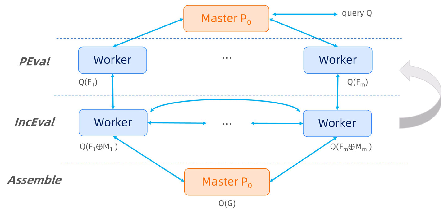
The analytical engine in GraphScope derives from GRAPE, a graph processing system proposed on SIGMOD-2017. GRAPE differs from prior systems in its ability to parallelize sequential graph algorithms as a whole. In GRAPE, sequential algorithms can be easily “plugged into” with only minor changes and get parallelized to handle large graphs efficiently. In addition to the ease of programming, GRAPE is designed to be highly efficient and flexible, to cope the scale, variety and complexity from real-life graph applications.
Built-in Algorithms
GraphScope analytical engine provides many common used algorithms, including connectivity and path analysis, community detection, centrality computations.
Built-in algorithms can be easily invoked over loaded graphs. For example,
import graphscope
from graphscope import pagerank
from graphscope import lpa

g = graphscope.g()
# algorithms defined on property graph can be invoked directly.
result = lpa(g)

# some other algorithms may only support evaluate on simple graph
# hence we need to generate one by selecting a kind of vertices and edges.
simple_g = g.project(vertices={"users": []}, edges={"follows": []})
result_pr = pagerank(simple_g)
A full-list of builtin algorithms is shown as below. Whether an algorithm supports property graph or not is described in its docstring.
The list is continuously growing.
Result Processing
When finish a computation, the results are wrapped as Context and preserved on the distributed machines.
Users may want to fetch the results to the client, or write to cloud storage or distributed file systems.
There is a list of supported method to retrieve the results.
# fetch to data structures
result_pr.to_numpy()
result_pr.to_dataframe()

# or write to hdfs or oss, or local (local means the path is relative to the pods)
result_pr.output("hdfs://output")
result_pr.output("oss://id:key@endpoint/bucket/object")
result_pr.output("file:///tmp/path")

# or write to client local
result_pr.output_to_client("local_filename")

# or seal to vineyard
result_pr.to_vineyard_dataframe()
result_pr.to_vineyard_numpy()
In addition, as shown in the Getting Started, computation results can add back to the graph as a new property (column) of the vertices(edges).
simple_g = g.project(vertices={"paper": []}, edges={"sites": []})
ret = graphscope.kcore(simple_g, k=5)

# add the results as new columns to the citation graph, the column name is 'kcore'
subgraph = sub_graph.add_column(ret, {'kcore': 'r'})
Users may assign a Selector to define which parts of the results to write. A selector specifies which part of the result to preserve. Similarly, the graph data can also be a part of the result, e.g., the vertex id. We reserve three keywords for selectors. r represents the result, v and e for vertices and edges, respectively. Here are some examples for selectors on result processing.
# get the results on the vertex
result_pr.to_numpy('r')

# to dataframe,
# using the `id` of vertices (`v.id`) as a column named df_v
# using the `data` of v (`v.data`) as a column named df_vd
# and using the result (`r`) as a column named df_result
result_pr.to_dataframe({'df_v': 'v.id', 'df_vd': 'v.data', 'df_result': 'r'})

# for results on property graph
# using `:` as a label selector for v and e
# using the id for vertices labeled with label0 (`v:label0.id`) as column `id`
# using the property0 written on vertices with label0 as column `result`
result.output(fd='hdfs:///gs_data/output', \
        selector={'id': 'v:label0.id', 'result': 'r:label0.property0'})
Writing Your Own Algorithms in PIE
Users may write their own algorithms if the built-in algorithms do not meet their needs. graphscope enables users to write algorithms in the PIE programming model in a pure Python mode.
To implement this, a user just need to fulfill this class.
from graphscope.analytical.udf import pie
from graphscope.framework.app import AppAssets

@pie
class YourAlgorithm(AppAssets):
    @staticmethod
    def Init(frag, context):
        pass

    @staticmethod
    def PEval(frag, context):
        pass

    @staticmethod
    def IncEval(frag, context):
        pass
As shown in the code, users need to implement a class decorated with @pie and provides three sequential graph functions. In the class, the Init is a function to set the initial status. PEval is a sequential method for partial evaluation, and IncEval is a sequential function for incremental evaluation over the partitioned fragment. The full API of fragment can be found in Cython SDK API.
Let’s take SSSP as example, a user defined SSSP in PIE model may be like this.
from graphscope.analytical.udf import pie
from graphscope.framework.app import AppAssets

@pie(vd_type="double", md_type="double")
class SSSP_PIE(AppAssets):
    @staticmethod
    def Init(frag, context):
        v_label_num = frag.vertex_label_num()
        for v_label_id in range(v_label_num):
            nodes = frag.nodes(v_label_id)
            context.init_value(
                nodes, v_label_id, 1000000000.0, PIEAggregateType.kMinAggregate
            )
            context.register_sync_buffer(v_label_id, MessageStrategy.kSyncOnOuterVertex)

    @staticmethod
    def PEval(frag, context):
        src = int(context.get_config(b"src"))
        graphscope.declare(graphscope.Vertex, source)
        native_source = False
        v_label_num = frag.vertex_label_num()
        for v_label_id in range(v_label_num):
            if frag.get_inner_node(v_label_id, src, source):
                native_source = True
                break
        if native_source:
            context.set_node_value(source, 0)
        else:
            return
        e_label_num = frag.edge_label_num()
        for e_label_id in range(e_label_num):
            edges = frag.get_outgoing_edges(source, e_label_id)
            for e in edges:
                dst = e.neighbor()
                distv = e.get_int(2)
                if context.get_node_value(dst) > distv:
                    context.set_node_value(dst, distv)

    @staticmethod
    def IncEval(frag, context):
        v_label_num = frag.vertex_label_num()
        e_label_num = frag.edge_label_num()
        for v_label_id in range(v_label_num):
            iv = frag.inner_nodes(v_label_id)
            for v in iv:
                v_dist = context.get_node_value(v)
                for e_label_id in range(e_label_num):
                    es = frag.get_outgoing_edges(v, e_label_id)
                    for e in es:
                        u = e.neighbor()
                        u_dist = v_dist + e.get_int(2)
                        if context.get_node_value(u) > u_dist:
                            context.set_node_value(u, u_dist)
As shown in the code, users only need to design and implement sequential algorithm over a fragment, rather than considering the communication and message passing in the distributed setting. In this case, the classic dijkstra algorithm and its incremental version works for large graphs partitioned on a cluster.
Writing Algorithms in Pregel
In addition to the sub-graph based PIE model, graphscope supports vertex-centric Pregel model as well. You may develop an algorithms in Pregel model by implementing this.
from graphscope.analytical.udf import pregel
from graphscope.framework.app import AppAssets

@pregel(vd_type='double', md_type='double')
class YourPregelAlgorithm(AppAssets):

    @staticmethod
    def Init(v, context):
        pass

    @staticmethod
    def Compute(messages, v, context):
        pass

    @staticmethod
    def Combine(messages):
        pass
Differ from the PIE model, the decorator for this class is @pregel.
And the functions to be implemented is defined on vertex, rather than the fragment.
Take SSSP as example, the algorithm in Pregel model looks like this.
from graphscope.analytical.udf import pregel
from graphscope.framework.app import AppAssets

# decorator, and assign the types for vertex data, message data.
@pregel(vd_type='double', md_type='double')
class SSSP_Pregel(AppAssets):

    @staticmethod
    def Init(v, context):
        v.set_value(1000000000.0)

    @staticmethod
    def Compute(messages, v, context):
        src_id = context.get_config(b"src")
        cur_dist = v.value()
        new_dist = 1000000000.0
        if v.id() == src_id:
            new_dist = 0
        for message in messages:
            new_dist = min(message, new_dist)
        if new_dist < cur_dist:
            v.set_value(new_dist)
            for e_label_id in range(context.edge_label_num()):
                edges = v.outgoing_edges(e_label_id)
                for e in edges:
                    v.send(e.vertex(), new_dist + e.get_int(2))
        v.vote_to_halt()

    @staticmethod
    def Combine(messages):
        ret = 1000000000.0
        for m in messages:
            ret = min(ret, m)
        return ret
Using math.h Functions in Algorithms
GraphScope supports using C functions from math.h in user-defined algorithms,
via the context.math interface. E.g.,
@staticmethod
def Init(v, context):
    v.set_value(context.math.sin(1000000000.0 * context.math.M_PI))
will be translated to the following efficient C code
... Init(...)

    v.set_value(sin(1000000000.0 * M_PI));
Run Your Own Algorithms
To run your own algorithms, you may trigger it in place where you defined it.
import graphscope

sess = graphscope.session()
g = sess.g()

# load my algorithm
my_app = SSSP_Pregel()

# run my algorithm over a graph and get the result.
# Here the `src` is correspondent to the `context.get_config(b"src")`
ret = my_app(g, src="0")
After developing and testing, you may want to save it for the future use.
SSSP_Pregel.to_gar("file:///var/graphscope/udf/my_sssp_pregel.gar")
Later, you can load your own algorithm from the gar package.
import graphscope

g = graphscope.g()

# load my algorithm from a gar package
my_app = load_app('file:///var/graphscope/udf/my_sssp_pregel.gar')

# run my algorithm over a graph and get the result.
ret = my_app(g, src="0")
Writing Your Own Algorithms In Java
If you are a Java programmer, then you may want to implement your graph algorithm in Java, and
run it on GraphScope analytical engine.
Step 0: Get grape-jdk
First, you will need grape-jdk installed on your developing environment. We will support downloading/installing grape-jdk
from maven central repositories in the future, however, currently you need to build from source.
Please follow About Grape JDK for building grape-jdk from source.
After installing grape-jdk, you can include it as dependency in your maven project. You shall add classifier shaded to use the jar which includes all necessary dependencies.
<dependency>
  <groupId>com.alibaba.graphscope</groupId>
  <artifactId>grape-jdk</artifactId>
  <version>0.1</version>
  <classifier>shaded</classifier>
</dependency>
Step 1: Develop your graph algorithm in Java
- You shall implement your algorithm in PIE programming model, and your app shall inherit
com.alibaba.graphscope.app.PropertyDefaultAppBaseif it works on a property graph, orcom.alibaba.graphscope.app.ProjectedDefaultAppBasein case it works on a projected graph.Here we present a simple app which traverse all vertices and edges on a property graph.
public class PropertyTraverseVertexData implements PropertyDefaultAppBase<Long, PropertyTraverseVertexDataContext> {
    static private int propertyId = 0;

    @Override
    public void PEval(ArrowFragment<Long> fragment, PropertyDefaultContextBase<Long> context,
            PropertyMessageManager messageManager) {
        PropertyTraverseVertexDataContext ctx = (PropertyTraverseVertexDataContext) context;
        for (int i = 0; i < fragment.vertexLabelNum(); ++i) {
            VertexRange<Long> innerVertices = fragment.innerVertices(i);
            for (Vertex<Long> vertex : innerVertices.locals()) {
                for (int j = 0; j < fragment.edgeLabelNum(); ++j) {
                    PropertyAdjList<Long> adjList = fragment.getOutgoingAdjList(vertex, j);
                    for (PropertyNbr<Long> nbr : adjList.iterator()) {
                        Vertex<Long> dst = nbr.neighbor();
                        double edgeData = nbr.getDouble(propertyId);
                    }
                }
            }
        }
    }

    @Override
    public void IncEval(ArrowFragment<Long> fragment, PropertyDefaultContextBase<Long> context,
            PropertyMessageManager messageManager) {
        PropertyTraverseVertexDataContext ctx = (PropertyTraverseVertexDataContext) context;
        if (ctx.step >= ctx.maxStep) {
            return;
        }
        for (int i = 0; i < fragment.vertexLabelNum(); ++i) {
            VertexRange<Long> innerVertices = fragment.innerVertices(i);
            for (Vertex<Long> vertex : innerVertices.locals()) {
                for (int j = 0; j < fragment.edgeLabelNum(); ++j) {
                    PropertyAdjList<Long> adjList = fragment.getOutgoingAdjList(vertex, j);
                    for (PropertyNbr<Long> nbr : adjList.iterator()) {
                        Vertex<Long> dst = nbr.neighbor();
                        double edgeData = nbr.getDouble(propertyId);
                    }
                }
            }
        }
        messageManager.ForceContinue();
    }
}
Step 2: Pack to jar and submit to GraphScope
To run your algorithms on GraphScope analytical engine, first you need to pack your algorithms in a jar.
To address the jar dependencies issue, we need you to pack with dependencies included. For example, you can
used maven plugin maven-shade-pluging.
<plugin>
    <groupId>org.apache.maven.plugins</groupId>
    <artifactId>maven-shade-plugin</artifactId>
</plugin>
You will need python client to run a java app. A simple jar can contains serveral app implementation,
and you need to specify the app you want in this run.
import graphscope
from graphscope import JavaApp
graphscope.set_option(show_log=True)
"""Or lauch session in k8s cluster"""
sess = graphscope.session(cluster_type='hosts')

graph = sess.g()
graph = sess.g(directed=False)
graph = graph.add_vertices("gstest/property/p2p-31_property_v_0", label="person")
graph = graph.add_edges("gstest/property/p2p-31_property_e_0", label="knows")

sssp1=JavaApp(
    full_jar_path="full/path/to/your/packed/jar",
    java_app_class="fullly/qualified/class/name/of/your/app",
)
ctx2=sssp1(graph,src=6)

graph = graph.project(vertices={"person": ['id']}, edges={"knows": ["dist"]})
sssp3=JavaApp(
    full_jar_path="full/path/to/your/packed/jar",
    java_app_class="app/on/projected/graph",
)
ctx3=sssp3(graph,src=6)

ctx.to_numpy("r:label0.dist_0")
After computation, you can obtain the results stored in context with the help of Context.
Publications
Wenfei Fan, Jingbo Xu, Wenyuan Yu, Jingren Zhou, Xiaojian Luo, Ping Lu, Qiang Yin, Yang Cao, and Ruiqi Xu. Parallelizing Sequential Graph Computations., ACM Transactions on Database Systems (TODS) 43(4): 18:1-18:39.
Wenfei Fan, Jingbo Xu, Yinghui Wu, Wenyuan Yu, Jiaxin Jiang. GRAPE: Parallelizing Sequential Graph Computations., The 43rd International Conference on Very Large Data Bases (VLDB), demo, 2017 (the Best Demo Award).
Wenfei Fan, Jingbo Xu, Yinghui Wu, Wenyuan Yu, Jiaxin Jiang, Zeyu Zheng, Bohan Zhang, Yang Cao, and Chao Tian. Parallelizing Sequential Graph Computations., ACM SIG Conference on Management of Data (SIGMOD), 2017 (the Best Paper Award).
Glossory
LoadStrategy
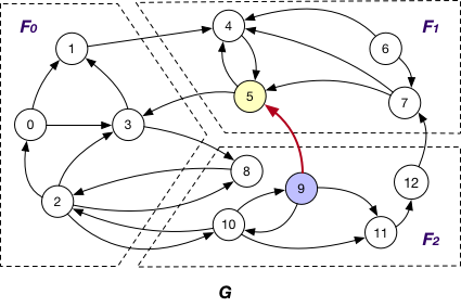
There are three ways to maintain the nodes crossing different fragments in GraphScope analytical engine.
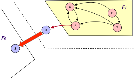
OnlyOut
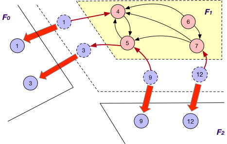
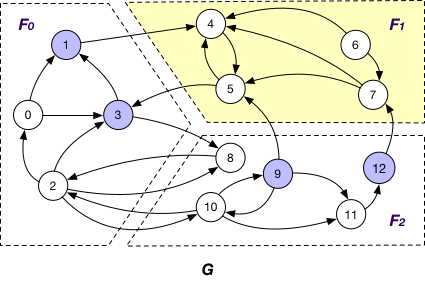
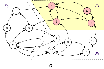
Each fragment Fi maintains “local” nodes v and a set of “mirrors” for nodes v’ in other fragments such that there exists an edge (v, v’). For instance, in addition to local nodes {4, 5, 6, 7}, F1 in graph G also stores a “mirror” node 3 and the edge (5, 3) when using OnlyOut strategy, as shown below.
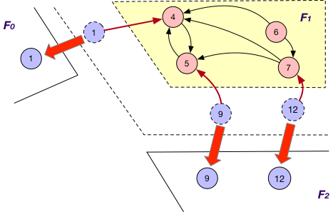
OnlyIn
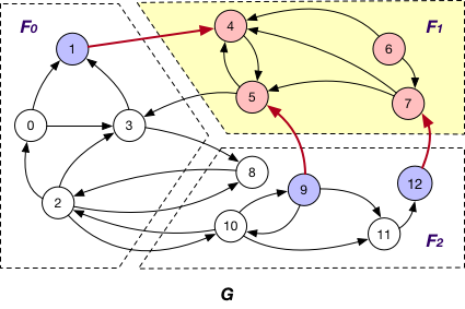
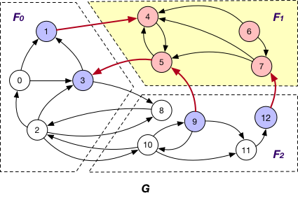
Under this case, each fragment Fi maintains “local” nodes v and a set of “mirrors” for nodes v’ in other fragments such that there exists an edge (v’, v). In graph G, F1 maintains “mirror” nodes {1, 9, 12} besides its local nodes.
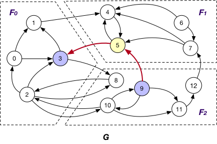
BothInOut
Each fragment Fi maintains “local” nodes v and a set of “mirrors” for nodes v’ in other fragments such that there exists an edge (v, v’) or (v’, v). Hence, in graph G, “mirror” nodes {1, 3, 9, 12} are stored in F1 when BothInOut is applied.
PartitionStrategy
Edge Cut
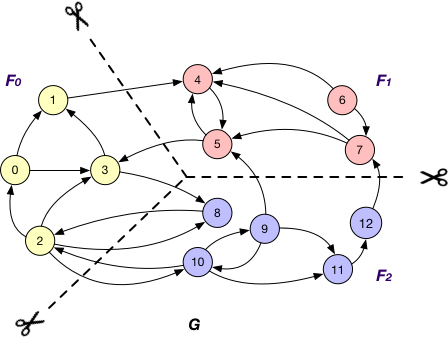
An edge cut partitioning splits vertices of a graph into roughly equal size clusters. The edges are stored in the same cluster as one or both of its endpoints. Edges with endpoints distributed across different clusters are crossing edges.
Vertex Cut
A vertex-cut partitioning divides edges of a graph into roughly equal size fragments. The vertices that hold the endpoints of an edge are also placed in the same fragment as the edge itself. A vertex has to be replicated when its adjacent edges are distributed across different fragments.
Vertices on GraphScope analytical engine
A node v is referred to as an
OuterVertex
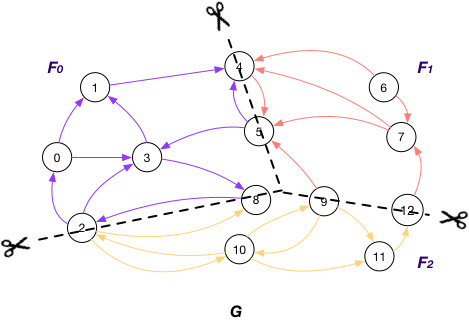
OuterVertex of fragment Fi if it resides at another fragment Fj and there exists a node v’ in Fi such that (v, v’) or (v’, v) is an edge; e.g., nodes {1, 3, 9, 12} are OuterVertex of fragment F1 in graph G;
InnerVertex
InnerVertex of fragment Fi if it is distributed to Fi; e.g. nodes {4, 5, 6, 7} are InnerVertex of fragment F1 in G;
InnerVertexWithOutgoingEdge
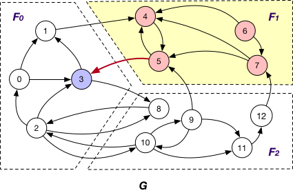
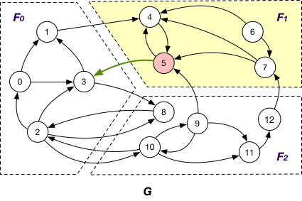
InnerVertexWithOutgoingEdge of fragment Fi if it is stored in Fi and has an adjacent edge (v, v’) outcoming to a node v’ in another fragment Fj; e.g., node 5 is an InnerVertexWithOutgoingEdge of F1 in G with the outgoing edge (5, 3);
InnerVertexWithIncomingEdge
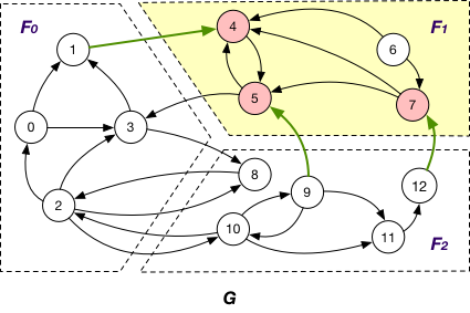
InnerVertexWithIncomingEdge of fragment Fi if it is maintained in Fi has an adjacent edge (v’, v) incoming from a node v’ in another fragment Fj; e.g., nodes {4, 5, 7} are InnerVertexWithIncomingEdge of F1 in G, and (1, 4), (9, 5), and (12, 7) are corresponding incoming edges.
MessageStrategy
Below are some message passing and synchronization strategies adopted by GraphScope analytical engine.
AlongOutgoingEdgeToOuterVertex
Here the message is passed along crossing edges from InnerVertexWithOutgoingEdge to OuterVertex. For instance, the message is passed from node 5 to 3 in graph G.
AlongIncomingEdgeToOuterVertex
Under this case, the message is passed along crossing edges from InnerVertexWithIncomingEdge to OuterVertex. For example, the message is passed from node 5 to 9 in graph G.
AlongEdgeToOuterVertex
Each message is passed along crossing edges from nodes that are both InnerVertexWithIncomingEdge and InnerVertexWithOutgoingEdge to OuterVertex, e.g., messages are passed from node 5 to 3 and 9 and vice versa in graph G.
SyncOnOuterVertexAsTarget
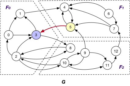
It is applied in company with the OnlyOut loading strategy. Here each fragment Fi sends the states of its “mirror” node of OuterVertex v to Fj that v resides, if there exists edge (v’, v) and v’ is “local” node of Fi, for synchronizing different states of v. For instance, the state of “mirror” node 3 is sent from F1 to F0 for synchronization at F0.
SyncOnOuterVertexAsSource
It is applied together with the OnlyIn loading strategy. Similar to SyncStateOnOuterVertexAsTarget, each fragment Fi sends the states of its “mirror” nodes v to the corresponding fragments for synchronization. The difference is that for each such “mirror”, there exists outgoing edge (v, v’) to certain “local” node v’ of Fi. For example, the states of “mirror” nodes 1, 9, and 12 are sent from F1 to F0 and F2 for synchronization with other states.
SyncOnOuterVertex
This is applied together with the BothInOut loading strategy. Under this case, each fragment Fi sends the states of all its “mirror” nodes v to the corresponding fragments for synchronization, regardless of the directions of edges adjacent to v, e.g., the states of “mirror” nodes 1, 3, 9 and 12 are sent from F1 to F0 and F2 for further synchronization.